Quantum includes the ability to perform symbolic math– a style of computing called computational algebra. This is a mode of calculation distinct from numeric computation. These types of systems are able to perform algebraic manipulation on abstract symbols. In other words, the system can perform algebraic manipulation in the same way a human would. When used in a network of complex mathematical relationships this can offer a significant source of benefits for computational efficiency due to algebraic simplification and cancellation.

Symbolic v.s. Numeric Computation

Computational algebra systems (CAS) are not new but they are a niche in computing typically occupied by those in academia. If you aren’t familiar with what a CAS does, I’ll provide a brief summary. First, let’s contrast a CAS with standard numeric computation. Numeric computation is made possible by the von Neumann architecture, a type of Turing machine. These machines use input variables to collect values and hold them in memory where a processor can read and write to perform calculations. All modern computers operate this way. If one wanted to program such a system to calculate an integral of an arbitrary continuous function, one might start with defining the procedure as a Riemann sum. It would loop over discrete intervals in the domain, calculate the value of the function at the midpoint of that interval, and multiply that with the width of the interval. The smaller the intervals, the more accurate the result would be.

By contrast, a CAS is able to find an analytical solution to the integral and simply use that to provide the exact solution. For example, suppose your function is $f(x) = x$. A CAS would be able to provide the integrated form of $f$ as $F(x) = \frac{1}{2}x^2$. To illustrate the syntax:

>>> from sympy import *
>>> x = Symbol('x')
>>> print(integrate(x))
x**2/2

From there, it’s a simple matter of plugging in your domain limits to find the area under the curve. The reader may be surprised to learn that obtaining a numeric solution in a symbolic system is often slower than an optimized numeric method. This is because a CAS is a set of algorithms that must be defined within the architecture designed for numeric calculation and therefore the CAS spends a lot of its time trying to get to the analytical solution. It’s not hard to imagine that an algorithm to express symbolic relationships in a numeric system will inherently be more expensive than a numeric algorithm that can directly carry out it’s purpose on the same architecture. In a symbolic system, numbers themselves become abstract symbols and equations must undergo a translation process in order to generate a numeric result. Despite being a slower method, the CAS has a very important role to play in optimizing a numeric system. If you’ve realized that a CAS needs only to calculate the analytical solution once as the up-front cost, then you’re on the right track.

Quantum Disentanglement

The effect of a CAS on a network graph of symbolic expressions is to further disentangle node dependencies. Take the following expression and its graph representation as an example: \[ \frac{x^2+2x+1}{x^2+x} \]

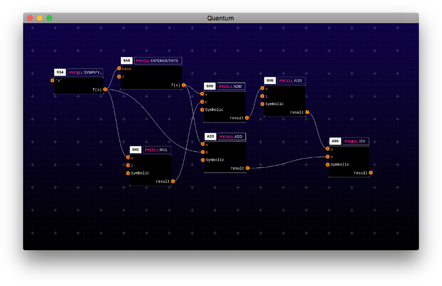
It should be clear that there is a topological hierarchy which imposes a calculation dependency. For example, node A20 is dependent on 98A and node 90G is dependent on 98A and 9HC. Both A20 and 90G are independent from each other, so they could be calculated concurrently, however, with symbolic representation, we can actually remove all dependencies!

If each node keeps track of its symbolic state as it is being connected to upstream nodes, then each node would be independent of the calculation being performed upstream. For example, 98A would carry out the calculation $x^2$ while 90G would carry out the calculation $x^2 + 2x$ and it could do so independent of the calculation occurring at 98A. This can be a very effective strategy if deployed correctly. You may notice that we are now making the same calculation in multiple nodes, which means we are increasing the total amount of processing work. For example, we calculate $x^2$ in both 98A and 90G. So although we’ve increased the parallelism of our system, each processor must now do more work.

Efficiency

The advantage of arbitrary and unlimited parallelism isn’t in making the whole system 100% parallel, but rather by providing the option for it to load balance in an intelligent way. It allows the system to utilize all processes at all times because there will always be a node in the processing queue ready to go. At the same time, if upstream values have already been processed, a node that is scheduled for processing need not recalculate that portion, but rather reuse the value from the upstream result. Furthermore, we can target particular cells for calculation without needing to to calculate the ones we’re not interested in.

Another useful consequence is the potential for simplification. For example, if we are only interested in the end result of our equation and none of the intermediate values, then you may notice that the equation simplifies: \[ \frac{x^2+2x+1}{x^2+x} = 1 + \frac{1}{x} \]

Basic Example

One can imagine that in an actual model, $x$ may represent a function, perhaps a computationally expensive function. For the sake of being more concrete, suppose $x$ represents a discount factor calculation and we call it $g(t)$. In Python, we can use Sympy to express this symbolically as follows:

from sympy import *
g = Function('g')
expr = (g(t)**2 + 2*g(t) + 1)/(g(t)**2 + g(t))

Now we have a symbolic expression defined in variable expr. We can bind it to an actual function to calculate a result. Any manipulation of the symbolic representations will result in changes to the function calls. For the example, let’s bind the original unsimplified form of the equation to gn and the simplified form to fn. Once bound, these become callable objects. We can then time the two functions over 10000 iterations to observe the difference in calculation time.

# The interest function is included for completeness. You can pretend it's a table-lookup.
def rate(t):
    return 0.05

def discount(t):
    if t<=0:
        return 1
    else:
        return discount(t-1)*(1+rate(t))**(-1/12)

# We now create gn and fn as callable functions that bind the expression to the discount function.
# gn is bound to the original form of the expression
gn = lambdify(t, expr, {'g':discount})
# fn is bound to the simplified form
fn = lambdify(t, expr.simplify(), {'g':discount})

# We can now analyze the performance difference.
import timeit
print(f"simplified: {timeit.timeit('fn(100)', 'from __main__ import fn', number=10000)}")
print(f"original: {timeit.timeit('gn(100)', 'from __main__ import gn', number=10000)}")

simplified: 0.45651856798212975
original: 1.9525561300106347

What we’re doing here is mapping an actual function implementation to its symbolic representation with lambdify. The benefit here is we can now use sympy to manipulate function relationships in our model. We can create an expression that relates multiple functions, call simplify on that and reduce to a simpler form, then lambdify it to produce a calculation. For example, if we have a very complex expression that multiplies by the discount rate at one point and divides by it at another point, then these two operations cancel out when we symbolically simplify the expression and thus we are able to save computation cycles.

Symbolic Black and Scholes

Let us consider a more complex example of using symbolic math in a model implementation. In the Black and Scholes model, we’re often interested in the price sensitivities of options with respect to various parameters such as time or volatility. This would make a good example for how symbolic math can help us. I’ll first give a brief review of the classic Black and Scholes equations and cover how that might be implemented in pure Python using Sympy to provide symbolic representation. We can then break up the components of the Python implementation and put them into Quantum cells. We’ll wire up the cells in a Quantum circuit to examine the graph implementation.

Price of Non-dividend European Call Option

\[ C = S_{t} N{\left (d_{1} \right )} - N{\left (d_{2} \right )} K e^{- r \left(T - t\right)} \]

\[ d_1 = \frac{1}{\sigma \sqrt{T - t}} \left(\left(T - t\right) \left(r + \frac{\sigma^{2}}{2}\right) + \ln{\left (\frac{S_{t}}{K} \right )}\right) \]

\[ d_2 = \frac{1}{\sigma \sqrt{T - t}} \left(\left(T - t\right) \left(r + \frac{\sigma^{2}}{2}\right) + \ln{\left (\frac{S_{t}}{K} \right )}\right) - \sigma \sqrt{T - t} \]

Where:

• $C$ is the call option price
• $S_t$ is the price of the underlying security at time $t$
• $N()$ is the standard normal cumulative distribution function
• $K$ is the strike price of the underlying security
• $r$ is the risk-free rate
• $\sigma$ is the volatility (standard deviation) of the underlying security
• $\left(T-t\right)$ is the time to maturity of the option

To define this symbolically in Python, we would write:

import sympy as sp

#spot, strike, volatility, time, interest rate, time at expiry, d1, and d2
S, K, sigma, t, r, T, d1, d2 = sp.symbols('S_t,K,sigma,t,r,T,d_1,d_2')

#define a symbol to represent the normal CDF
N = sp.Function('N')

#Black and Scholes price
C = S * N(d1) - N(d2) * K * sp.exp(-r * (T-t))

We’ve now created a symbolic expression for the call price. In order to turn this into a callable function, we’ll need to expand the $d_1$ and $d_2$ terms, then bind the $N$ to a callable normal function. We won’t need to define the normal CDF symbolically because sympy provides a normal CDF as part of its stats module. Continuing on…

from sympy.stats import Normal, cdf

#expanded d1 and d2 for substitution:
d1_sub = (sp.ln(S / K) + (r + sp.Rational(1,2) * sigma ** 2) * (T-t)) / (sigma * sp.sqrt(T-t))
d2_sub = d1 - sigma * sp.sqrt(T-t)

#instance a standard normal distribution:
Norm = Normal('N',0.0, 1.0)

#define the long form b-s equation with all substitutions:
bs = C.subs(N, cdf(Norm)).subs(d2, d2_sub).subs(d1, d1_sub)

In the last line, you see an example of sympy’s subs function. It is an algebraic operation that performs symbolic substitution of various terms in the expression C. This produces the expanded form of the call price equation that we will turn into a callable function. Continuing on…

#Callable function for black and scholes price:
#example usage: bs_calc(100, 98, 0.15, 0, 0.03, 0.5)
bs_calc = sp.lambdify((S, K, sigma, t, r, T), bs)

We can also take the derivatives and turn those into callable functions as well!

#1st Order Greeks
delta = sp.lambdify((S, K, sigma, t, r, T),bs.diff(S))
vega = sp.lambdify((S, K, sigma, t, r, T),bs.diff(sigma))
theta = sp.lambdify((S, K, sigma, t, r, T),bs.diff(t))
rho = sp.lambdify((S, K, sigma, t, r, T),bs.diff(r))

#2nd Order Greeks
gamma = sp.lambdify((S, K, sigma, t, r, T),bs.diff(S,S))
vanna = sp.lambdify((S, K, sigma, t, r, T),bs.diff(S,sigma))
vomma = sp.lambdify((S, K, sigma, t, r, T),bs.diff(sigma,sigma))
charm = sp.lambdify((S, K, sigma, t, r, T),bs.diff(S,t))