
Working with Pandas in Quantum
I came across a tutorial on working with the modern Pandas API here. If you’re like me when working in Pandas, you have multiple web browser windows open containing various searches for Pandas syntax because I can never remember how to use the Pandas functions. Pandas is a great candidate for implementation in a graph processing network since graph processors do not require you to remember syntax. Working with dataframes, you often need multiple steps in your data wrangling and you are often reusing results of prior steps in later steps. As a result, I decided to write a series of posts that parallel this tutorial, however, I’ll also be using the posts to demonstrate how easy it is to wrap Pandas functions into PyCells.
Indexing
As mentioned in the tutorial, you can get rows from a dataframe by using the
loc and iloc methods. The loc function allows you to select rows or
columns by label when your indexes are labels. The iloc function allows you to
select rows and columns by their position. Here’s the code I used for wrapping
these into cells:
class Iloc(Custom):
    required = ['data']

    def __init__(self):
        self.inputs = {'axis0': None, 'axis1': None, 'data': None}
        self.outputs = {'dataframe': None}

    @data_process
    def iloc(self, h5):
        df = None
        if self.inputs['axis1'] is None:
            df = h5.df.iloc[self.inputs['axis0']]
        else:
            df = h5.df.iloc[self.inputs['axis0'], self.inputs['axis1']]
        return df

    def process(self):
        self.outputs['dataframe'] = self.iloc(self.inputs['data'])
        return super().process()
As you can see, I am subclassing the Custom class type that is provided by
PyCell and I am using the data_process decorator on my iloc function. If
you want to learn more about these aspects of the code, click through to the
documentation.
In the __init__ function, you will see that we define our input and output
sockets. These are defined as dictionaries and the keys will become the socket
names when Quantum spawns the cell. To get started building your own cell, you
can follow the template provided in the cookbook.
You can define whatever functions you need in the cell. In this example, I’ve
defined the iloc function which will be used in the process function. The
process function is a reserved name and gets called when Quantum executes the
cell.
The implementation of loc is pretty much exactly the same except that we
replace the h5.df.iloc call by h5.df.loc. Pretty simple. I add these to
the PyCell registry dictionary (within the dataframe_cell.py file) like so:
registry += [
    {
    'name': 'ILoc',
    'module': 'PyCell.dataframe_cell',
    'categories': ['Data', 'Modify']
    },
    {
    'name': 'Loc',
    'module': 'PyCell.dataframe_cell',
    'categories': ['Data', 'Modify']
    }
]
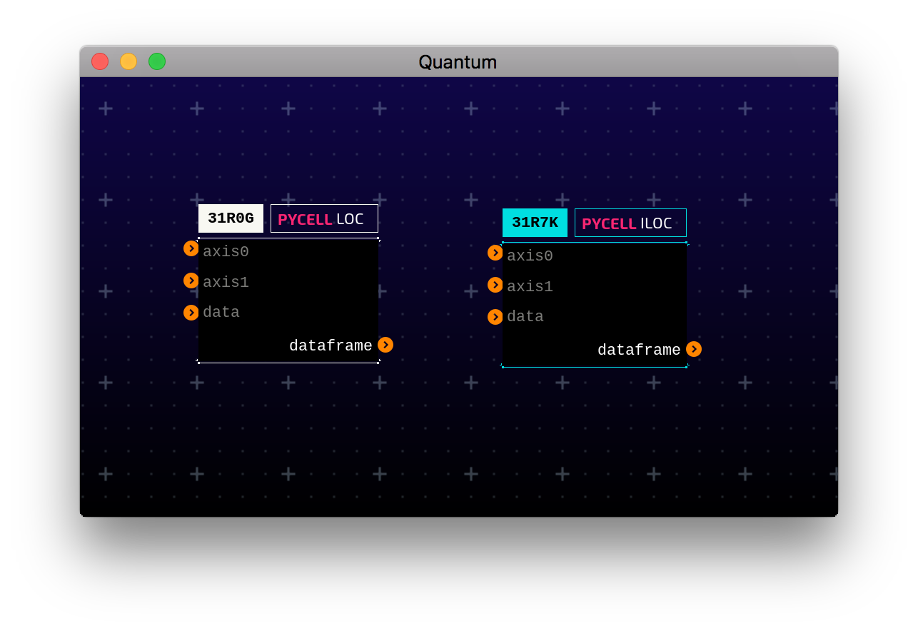
Once this is done, you will have access to these new cells in Quantum’s
contextual menu under Data>Modify>Iloc and Data>Modify>Loc. This is
what the cells should look like:
Modify a Dataframe
Let’s take a look at how we can use Quantum to manipulate our data. I’ll be using the following dataset:
df = pd.read_csv('tesla-sentiment.csv')
df.tail()
| Date | sentiment | influence | Open | High | Low | Close | Volume | |
|---|---|---|---|---|---|---|---|---|
| 281 | 2017-03-30 11:00:00-07:00 | 0.27 | 24 | 278.26 | 278.75 | 278.20 | 278.61 | 79532.0 |
| 282 | 2017-03-30 11:30:00-07:00 | 0.22 | 122 | 278.68 | 278.78 | 277.47 | 277.87 | 125126.0 |
| 283 | 2017-03-30 12:00:00-07:00 | 0.19 | 21 | 277.89 | 278.18 | 277.45 | 277.89 | 102393.0 |
| 284 | 2017-03-30 12:30:00-07:00 | 0.17 | 53 | 277.91 | 278.35 | 277.47 | 278.00 | 273989.0 |
| 285 | 2017-03-30 13:00:00-07:00 | 0.21 | 45 | 278.00 | 278.01 | 277.72 | 277.92 | 91511.0 |
This represents stock data where the Open, High, Low, Close represents prices for the time intervals found in Date. The meaning of other fields are unimportant for this example.
I’ll demonstrate how to perform the following manipulation:
df.loc[df['High']>279, 'High'] = df.loc[df['High']>279, 'High']/10
What we are doing is dividing any prices in the ‘High’ column by 10 if the price exceeds $279. Don’t ask me when you would ever need to do this to stock data.
We can accomplish this same task in Quantum with the Update cell. Here’s the
source code for Update:
class Update(Custom):
    required = ['dataframe', 'column', 'values']

    def __init__(self):
        self.return_msg_ = "Ready to update data."
        self.inputs = {'dataframe': None, 'rows': None, 'column': None,
                       'values': None}
        self.outputs = {'dataframe': None}

    @data_process
    def update(self, h5):
        assert isinstance(self.inputs['values'], H5), "Socket must be an H5."
        assert isinstance(self.inputs['rows'].df, pd.Series), \
            "Rows must be a series."
        df = h5.df
        df.loc[self.inputs['rows'].df, self.inputs['column']] = \
            self.inputs['values'].df
        return df

    def process(self):
        self.outputs['dataframe'] = self.update(self.inputs['dataframe'])
        self.return_msg_ = 'Data updated!'
        return super().process()
We use this cell like so:
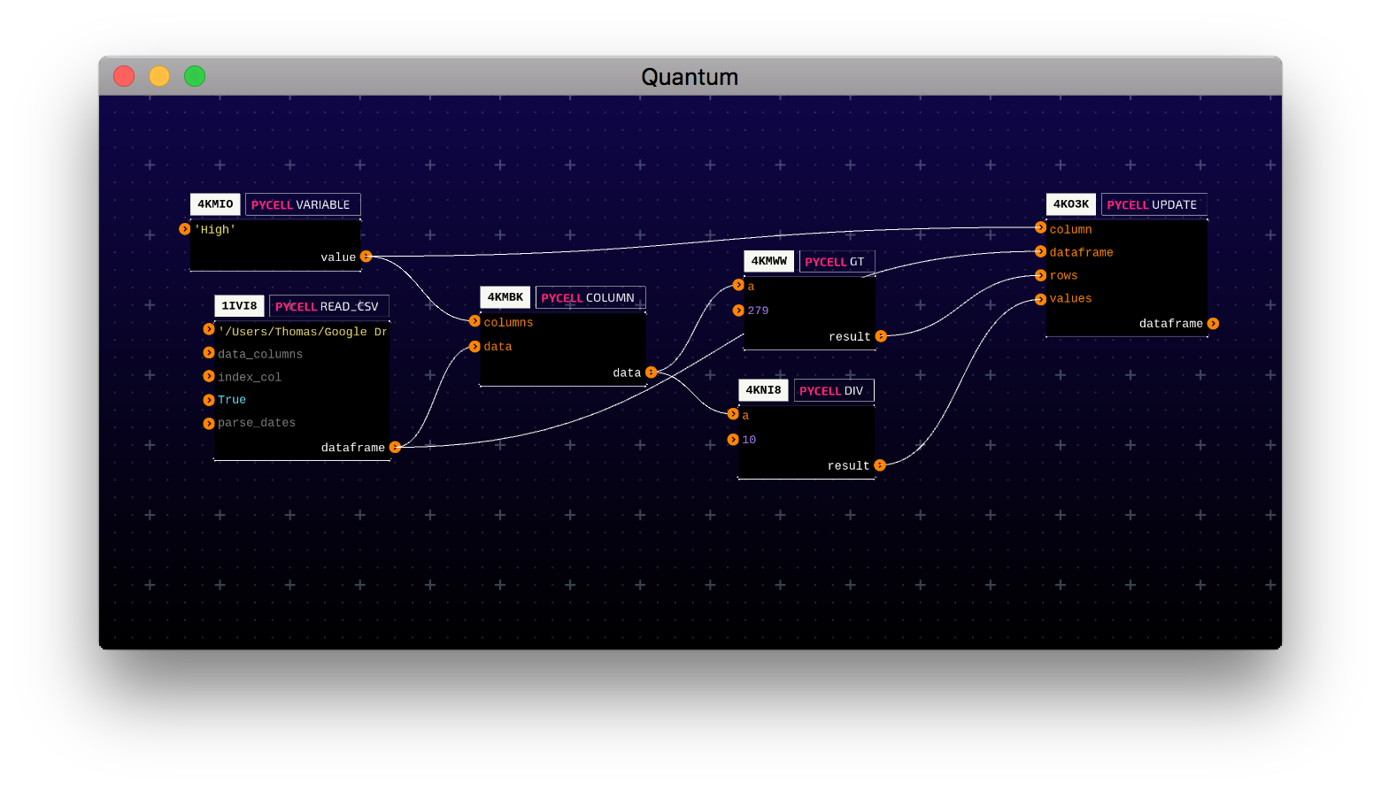
Here’s what’s going on in this circuit:
1IVI8: Read the csv file and turn it into a dataframe.4KMIO: Define a common variable to use in later cells.4KMBK: Grab a the data from the ‘High’ column.4KMWW: Filter the rows that are greater than 279.4KNI8: Calculate the values in ‘High’ divided by 10.4K03K: Set the values of the filtered rows to the calculated values.
Here’s the result:
| Date | sentiment | influence | Open | High | Low | Close | Volume | |
|---|---|---|---|---|---|---|---|---|
| 271 | 2017-03-29 13:00:00-07:00 | 0.02 | 114 | 277.36 | 277.380 | 277.12 | 277.38 | 56145.0 |
| 272 | 2017-03-30 06:30:00-07:00 | 0 | 52 | 278.04 | 28.200 | 277.21 | 281.45 | 1075623.0 |
| 273 | 2017-03-30 07:00:00-07:00 | 0.01 | 24 | 281.37 | 28.147 | 279.21 | 279.91 | 478321.0 |
| 274 | 2017-03-30 07:30:00-07:00 | 0 | 15 | 279.87 | 28.075 | 279.55 | 280.00 | 274664.0 |
| 275 | 2017-03-30 08:00:00-07:00 | 0.01 | 37 | 280.00 | 28.160 | 279.95 | 280.39 | 345942.0 |
| 276 | 2017-03-30 08:30:00-07:00 | 0.11 | 87 | 280.37 | 28.090 | 279.17 | 279.30 | 235248.0 |
| 277 | 2017-03-30 09:00:00-07:00 | 0.12 | 89 | 279.24 | 27.959 | 278.53 | 279.58 | 160264.0 |
| 278 | 2017-03-30 09:30:00-07:00 | 0.11 | 12 | 279.51 | 27.951 | 278.42 | 278.54 | 100704.0 |
| 279 | 2017-03-30 10:00:00-07:00 | 0.16 | 23 | 278.69 | 279.000 | 278.33 | 278.94 | 111686.0 |
| 280 | 2017-03-30 10:30:00-07:00 | 0.23 | 19 | 278.89 | 27.912 | 278.15 | 278.34 | 117323.0 |
| 281 | 2017-03-30 11:00:00-07:00 | 0.27 | 24 | 278.26 | 278.750 | 278.20 | 278.61 | 79532.0 |
| 282 | 2017-03-30 11:30:00-07:00 | 0.22 | 122 | 278.68 | 278.780 | 277.47 | 277.87 | 125126.0 |
| 283 | 2017-03-30 12:00:00-07:00 | 0.19 | 21 | 277.89 | 278.180 | 277.45 | 277.89 | 102393.0 |
| 284 | 2017-03-30 12:30:00-07:00 | 0.17 | 53 | 277.91 | 278.350 | 277.47 | 278.00 | 273989.0 |
| 285 | 2017-03-30 13:00:00-07:00 | 0.21 | 45 | 278.00 | 278.010 | 277.72 | 277.92 | 91511.0 |
Wrap Up
I’ll wrap up the post here. Hopefully, you saw how easy it is to define new cells for Quantum and how you can use Quantum for some basic data manipulation. In the next post I’ll cover some additional useful data manipulation cells as well as how you can visualize your data in Quantum. Thanks for reading!